The trajectory of the Moon's shadow is quite unusual during this event. The shadow axis passes to the far north where it barely grazes Earth's surface. In fact, the northern edge of the antumbra actually misses Earth so that one path limit is defined by the day/night terminator rather than by the shadow's upper edge. As a result, the track of annularity has a peculiar "D" shape that is nearly 1200 kilometers wide. Since the eclipse occurs just three weeks prior to the northern summer solstice, Earth's northern axis is pointed sunwards by 22.8ˇ. As seen from the Sun, the antumbral shadow actually passes between the North Pole and the terminator. As a consequence of this extraordinary geometry, the path of annularity runs from east to west rather than the more typical west to east.
The event transpires near the Moon's ascending node in Taurus five degrees north of Aldebaran. Since apogee occurs three days earlier (May 28 at 13 UT), the Moon's apparent diameter (29.6 arc-minutes) is still too small to completely cover the Sun (31.6 arc-minutes) resulting in an annular eclipse.
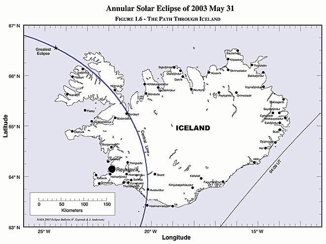
By 03:59 UT, the leading edge of the antumbra arrives along the southeastern coast of Iceland (Figure 1.6). Traveling with a ground velocity of 2 kilometers per second, the shadow sweeps across the entire North Atlantic nation in ten minutes. The shadow is so broad that the duration of the three and a half minute annular phase varies by less than 5 seconds across all of Iceland. The capital city of Reykjavik lies in the southwest corner of the country. Here, the Sun will stand 2ˇ high during the 3 minute 36 second annular phase. Unfortunately, the low altitude spectacle may be hidden from city dwellers by mountains lying to the northeast.
The instant of greatest eclipse occurs at 04:08:18 UT when the axis of the Moon's shadow passes closest to the center of Earth (gamma = +0.996). The length of annularity reaches its maximum duration of 3 minutes 37 seconds, the Sun's altitude is 3ˇ, and the antumbra's velocity is 1.06 km/s. At that time, the shadow's axis is just 60 kilometers northwest of Iceland.
After traversing the Denmark Strait, the highly elliptical antumbra bisects Greenland where over a third of the enormous island lies within the track (Figure 1.4). Crossing the ill-named land mass, the path width rapidly shrinks as the grazing antumbra begins its return to space. From Umanak, the Sun stands 3ˇ above the Arctic horizon during the 2 minute 24 second annular phase. Seven hundred kilometers to the south, Godthåb (Nuuk) lies completely outside the path and will not even witness a partial eclipse.
As it departs Greenland and crosses Baffin Bay, the shadow leaves Earth's surface at 04:31 UT. From start to finish, the antumbra sweeps over its entire path in a little under 47 minutes.
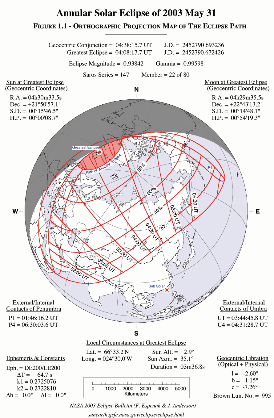
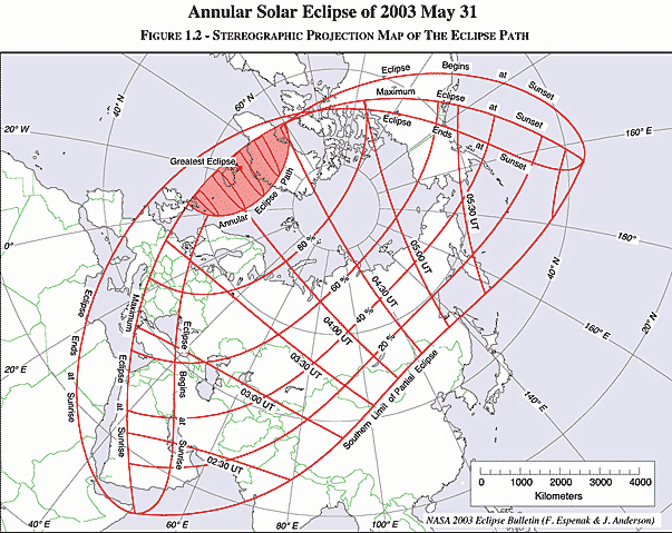
The limits of the Moon's penumbral shadow define the region of visibility of the partial eclipse. This saddle shaped region often covers more than half of Earth's daylight hemisphere and consists of several distinct zones or limits. At the southern boundary lies the limit of the penumbra's path. Great loops at the western and eastern extremes of the penumbra's path identify the areas where the eclipse begins/ends at sunrise and sunset, respectively. Bisecting the 'eclipse begins/ends at sunrise and sunset' loops is the curve of maximum eclipse at sunrise (western loop) and sunset (eastern loop). The exterior tangency points P1 and P4 mark the coordinates where the penumbral shadow first contacts (partial eclipse begins) and last contacts (partial eclipse ends) Earth's surface. The path of the antumbral shadow travels east to west and is shaded dark gray.
A curve of maximum eclipse is the locus of all points where the eclipse is at maximum at a given time. They are plotted at each half hour Universal Time (UT), and generally run in a north-south direction. The outline of the antumbral shadow is plotted every ten minutes in UT. Curves of constant eclipse magnitude delineate the locus of all points where the magnitude at maximum eclipse is constant. These curves run exclusively between the curves of maximum eclipse at sunrise and sunset. Furthermore, they are quasi-parallel to the southern penumbral limit. This limit may be thought of as a curve of constant magnitude of 0%, while adjacent curves are for magnitudes of 20%, 40%, 60% and 80%.
At the top of Figure 1.1, the Universal Time of geocentric conjunction between the Moon and Sun is given followed by the instant of greatest eclipse. The eclipse magnitude is given for greatest eclipse. For central eclipses (both total and annular), it is equivalent to the geocentric ratio of diameters of the Moon and Sun. Gamma is the minimum distance of the Moon's shadow axis from Earth's center in units of equatorial Earth radii. Finally, the Saros series number is given along with the eclipse's relative sequence in the series.
Figures 1.1 and 1.2 may be used to quickly determine the approximate time and magnitude of maximum eclipse at any location within the eclipse path.
The positions of larger cities and metropolitan areas are depicted as black dots. The size of each city is logarithmically proportional to its population using 1990 census data (Rand McNally, 1991). City data sellected from a geographic data base of over 90,000 cities are plotted to give as many locations as possible in the path of annularity. Local circumstances have been calculated for many of these positions and can be found in Tables 1.6 through 1.15.
Although no corrections have been made for center of figure or lunar limb profile, they have little or no effect at this scale. Altmospheric refraction has not been included because it depends on the atmospheric temperature-pressure profile, which cannot be predicted in advance. These maps are also available on the Web.
t = t1 - t0 (decimal hours) and
t0 = 4.000 TDT.
The polynomial Besselian elements were derived from a least-squares fit to elements rigorously calculated at five separate times over a six hour period centered at t0. Thus, the equation and elements are valid over the period 1.00 < t1 < 7.00 TDT.
Table 1.1 lists all contacts of penumbral and antumbral shadows with Earth. They include TDT times and geodetic coordinates with and without corrections for ΔT. The contacts are defined:
P1 - Instant of first external tangency of penumbral shadow cone with Earth's limb (partial eclipse begins)
P4 - Instant of last external tangency of penumbral shadow cone with Earth's limb (partial eclipse ends)
U1 - Instant of first external tangency of antumbral shadow cone with Earth's limb (annular eclipse begins)
U4 - Instant of last external tangency of antumbral shadow cone with Earth's limb (annular eclipse ends)
Similarly, the outhern extremes of the penumbral and antumbral paths, and extreme limits of the antumbral central line are given. The IAU (International Astronomical Union) longitude convention is used throughout this publication (i.e., for longitude, east is positive and west is negative; for latitude, north is positive and south is negative).
The path of the antumbral shadow is delineated at one minute intervals in Universal Time in Table 1.3. Coordinates of the terminator limit, the antumbral limit and the central line are listed to the nearest tenth of an arc-minute (~185 m at the Equator). The Sun's altitude, path width and antumbral duration are calculated for the central line position. Table 1.4 presents a physical ephemeris for the antumbral shadow at one minute intervals in UT. The central line coordinates are followed by the topocentric ratio of the apparent diameters of the Moon and Sun, the eclipse obscuration , and the Sun's altitude and azimuth at that instant. The antumbral shadow's instantaneous velocity with respect to Earth's surface are included. Finally, the central line duration of the antumbral phase is given.
Local circumstances for each central line position listed in Table 1.4 are presented in Table 1.5. The first three columns give the Universal Time of maximum eclipse, the central line duration of annularity and the altitude of the Sun at that instant. The following columns list each of the four eclipse contact times followed by their related contact position angles and the corresponding altitude of the Sun. The four contacts identify significant stages in the progress of the eclipse. They are defined as follows: First Contact - Instant of first external tangency between the Moon and Sun (partial eclipse begins)
Second Contact - Instant of first internal tangency between the Moon and Sun (central or antumbral eclipse begins; annular eclipse begins)
Third Contact - Instant of last internal tangency between the Moon and Sun (central or antumbral eclipse ends; annular eclipse ends)
Fourth Contact - Instant of last external tangency between the Moon and Sun (partial eclipse ends)
The position angles P and V identify the point along the Sun's disk where each contact occurs . Second and third contact altitudes are omitted since they are always within 1ˇ of the altitude at maximum eclipse.
Two additional columns are included if the location lies within the path of annularity The antumbral depth is a relative measure of a location's position with respect to the central line and path limits. It is a unitless parameter that is defined as:
where:
u| = | antumbral depth
| x | = | perpendicular distance from the shadow
axis (km)
| R | = | radius of the umbral shadow as it
intersects Earth's surface (km)
| |
The antumbral depth for a location varies from 0.0 to 1.0. A position at the path limits corresponds to a value of 0.0 while a position on the central line has a value of 1.0. The parameter can be used to quickly determine the corresponding central line duration. Thus, it is a useful tool for evaluating the trade-off in duration of a location's position relative to the central line. Using the location's duration and antumbral depth, the central line duration is calculated as:
where:
| D | = | duration of totality on the center line (seconds) |
| d | = | duration of totality at location (seconds) |
| u | = | antumbral depth |
The final column gives the duration of annularity. The effects of refraction have not been included in these calculations, nor have there been any corrections for center of figure or the lunar limb profile.
Locations were chosen based on general geographic distribution, population, and proximity to the path. The primary source for geographic coordinates is The New International Atlas (Rand McNally, 1991). Elevations for major cities were taken from Climates of the World (U. S. Dept. of Commerce, 1972). The city names and spellings presented here are for location purposes only and are not meant to be authoritative. They do not imply recognition of status of any location by the United States Government.
The Watts charts have been digitized and may be used to generate limb profiles for any libration. Ellipticity and libration corrections can be applied to refer the profile to the Moon's center of mass. Such a profile can then be used to correct eclipse predictions which have been generated using a mean lunar limb.
The lunar limb profile in Figure 1.7 includes corrections for center of mass and ellipticity [Morrison and Appleby, 1981]. It is generated for the central line at 04:05 UT, corresponding to central Iceland. The Moon's topocentric libration (physical + optical) is l=-2.46°, b=+1.28°, and the topocentric semi-diameters of the Sun and Moon are 945.5 and 888.2 arc-seconds, respectively. The Moon's angular velocity with respect to the Sun is 0.539 arc seconds per second.
The radial scale of the limb profile (bottom of Figure 1.7) is greatly exaggerated so that the true limb's departure from the mean lunar limb is readily apparent. The mean limb with respect to the center of figure of Watts' original data is shown (dashed) along with the mean limb with respect to the center of mass (solid). Note that all the predictions presented in this publication are calculated with respect to the latter limb unless otherwise noted. Position angles of various lunar features can be read using the protractor marks along the Moon's mean limb (center of mass). The position angles of second and third contact are clearly marked along with the north pole of the Moon's axis of rotation and the observer's zenith at mid-annularity. The dashed line identifies the contact point on the north limb corresponding to the path limit. To the upper left of the profile are the Sun's topocentric coordinates at maximum eclipse. They include the right ascension R.A., declination Dec., semi-diameter S.D. and horizontal parallax H.P. The corresponding topocentric coordinates for the Moon are to the upper right. Below and left of the profile are the geographic coordinates of the central line at 04:05 UT while the times of the eclipse contacts at that location appear to the lower right. Directly below the profile are the local circumstances at maximum eclipse. They include the Sun's altitude, azimuth, and central duration of annularity. The position angle of the path's southern limit axis is PA(N.Limit) and the angular velocity of the Moon with respect to the Sun is A.Vel.(M:S). At the bottom left are a number of parameters used in the predictions, and the topocentric lunar librations appear at the lower right.
In investigations where accurate contact times are needed, the lunar limb profile can be used to correct the nominal or mean limb predictions. For any given position angle, there will be a high mountain (annular eclipses) or a low valley (total eclipses) in the vicinity that ultimately determines the true instant of contact. The difference, in time, between the Sun's position when tangent to the contact point on the mean limb and tangent to the highest mountain (annular) or lowest valley (total) at actual contact is the desired correction to the predicted contact time. On the exaggerated radial scale of Figure 1.7, the Sun's limb can be represented as an epicyclic curve that is tangent to the mean lunar limb at the point of contact. Using the digitized Watts' datum, an analytical solution is straightforward and robust. Curves of corrections to the times of second and third contact for most position angles have been computer generated and plotted. The circular protractor scale at the center represents the nominal contact time using a mean lunar limb. The departure of the contact correction curves from this scale graphically illustrates the time correction to the mean predictions for any position angle as a result of the Moon's true limb profile. Time corrections external to the circular scale are added to the mean contact time; time corrections internal to the protractor are subtracted from the mean contact time. The magnitude of the time correction at a given position angle is measured using any of the four radial scales plotted at each cardinal point.
For example, Table 1.7 gives the following data for Reykjavik, Iceland:
Second Contact = 04:02:27.6 UT P2=254°
Third Contact = 04:06:03.5 UT P3=077°
Measuring the contact time corrections in Figure 1.7, the resulting contact times are:
C2=+3.2 seconds; Second Contact = 04:02:27.6 +3.2s = 04:02:30.8 UT
C3=-5.2 seconds; Third Contact = 04:06:03.5 -5.2s = 04:05:58.3 UT
The above corrected values are within 0.1 seconds of a rigorous calculation using the true limb profile.
Low pressure systems that develop and cross North America frequently turn to the northeast when they leave the continent, eventually ending their existence over the waters between Greenland and Iceland. This location is the home of the infamous Icelandic low, a semi-permanent depression that dictates not only the weather of its home island but also the meteorology of Britain and northern Europe. The low lies at the boundary of the cold Arctic airmass that lurks to the north and the warmer maritime climate that accompanies the Gulf Stream as it flows past Iceland in its clockwise circuit of the Atlantic.
The clash of warm and cold, both in the water and the atmosphere, generates a never-ending succession of mid-latitude frontal depressions that travel toward the British Isles. In Iceland, overcast skies with rain or snow are the norm, though precipitation amounts are not especially high. With its more southerly latitude, Scotland is able to tap occasionally into the drier air around the large high-pressure system that lingers near the Azores, and so the gloominess of north Atlantic weather is relieved occasionally by southerly breezes.
On the west coast winds tend to be lighter and more variable, but Davis Strait is a favorite destination for lows traveling across North America, and so the coast is visited by a steady series of disturbances. Cloud cover from these systems plus a persistent fog and low cloud that arises from the cool waters of Davis Strait combine to make this side of the island as nearly as cloudy as the east. Cloud cover statistics derived from satellite images are subject to a number of complications at Greenland's latitude, but the data do show a tendency to slightly less cloud along the west coast.
Air on the ice cap is much colder and denser than that in the lowlands and there is a steady downhill flow of cold air toward the coast from the interior known as a katabatic wind. Though generally light, the katabatic flow can exceed 100 km/h when channeled by terrain. It is most common on the steep eastern coast where they are known as Piteraq. Downslope winds such as these are warmed slightly and dried by compression and reach the coast as a cold but dry flow that can clear out some of the persistent clouds and bring good eclipse viewing conditions. Though they tend to be most common in the early morning, prediction is difficult, as they are highly variable from place to place.
On the west coast, a southeast Foehn wind often develops bringing warm dry weather as it descends from the mountain peaks. It is the Greenland counterpart of the Chinook of North America. Foehn winds may last for as long as three days and are frequently followed by precipitation. They are more efficient than katabatic winds in clearing out the persistent cloudiness along the coast. A cap cloud on the nearby mountains often heralds these winds.
For the hardiest (and wealthiest) eclipse travelers, the interior ice cap likely offers the best chances for clear eclipse viewing. Observations from the cap are few in number and tend to be more concerned with temperature and wind rather than cloud cover. Automatic satellite measurements of cloudiness are unreliable because of the bright ice background and the cold temperatures of the plateau. A Russian study using ten years of imagery from 1971 to 1980 measured very good sky conditions on the ice cap - 60 to 68% of the observations had clear skies or scattered clouds and only 12 to 18% were overcast. The clouds over the ice cap are also likely to be thinner than that on the coast as the cold air inland is not capable of holding as much moisture as that at lower altitude.
Southern regions are marginally more promising than those in the north, in large part because of the lower frequency of low cloud and fog. Prevailing winds tend to be from the easterly side, so that there is a modest downslope to the flow at Reykjavik and a consequent drying of the atmosphere. Clear skies are almost unknown, being less than 5% of observations at all stations save one. Because the eclipse occurs very early with the Sun only a few degrees above the northeast horizon, clear or scattered cloudiness is almost mandatory.
Satellite observations show a complex pattern of cloudiness around the island. The largest amounts are in the interior where the higher terrain promotes condensation in the atmosphere. The least cloud is found straddling the south shore, and reaches slightly inland near Keflavik and Eyrarbakki. On the basis of the available data, a location near Reykjavik would be the most promising, though a good eclipse expedition will follow the forecast rather than the climatology.
Once again the main culprit is the series of frequent frontal lows that pass across or north of the British Isles in their eastward migration. Virtually all of these lows will bring precipitation to northern Scotland but spring is the driest season with changeable weather and a chance of a dry spell. Inland areas tend to be cloudier than the coast, in large part because of the higher terrain that promotes the lifting of the moist air masses and their conversion into cloudy weather.
Fog is also common on the Scottish coast, but highly variable from place to place. From the data in Table 1.16, it appears that locations along Moray Firth (Inverness, Lossiemouth) have a relatively low incidence of fog while those exposed to the North Sea (Aberdeen) are much more likely to encounter it. This does not seem to have much of an impact on the probability of seeing the eclipse, for the stations within and near the track are all remarkably alike. On the Scottish mainland the most promising site is at Lossiemouth with a score of 0.34 while the least promising sites have a score of 0.30. These differences are too small to recommend one over another.
Rapid travel from site to site in Greenland is all but impossible unless by aircraft, and so the site selection must be on the basis of the climatology. The available evidence points to the interior ice cap as the best site by far on the entire track, but cost and opportunity will limit access there. Elsewhere in Greenland, the west coast holds more promise than the east, which dictates a site at Christianshab or Godhavn, the two largest communities within the annular zone. These sites are close to the observation sites of Egdesminde and Jacobshavn in Table 1.16. The Sun does not set on May 31 and so the lucky eclipse observer could be treated to a midnight sun in annular eclipse. A sequence of solar images with an eclipse just 2° above the north horizon would surely be one of the great eclipse photographs - except, perhaps, for those that can be obtained in Antarctica just six months later.