 |
Documentation > SXT Observation Notes > this page |
Image name: Photon_Transfer_Sept_98.png (click image to enlarge)
Image size: 111.329 KB (962x640)
Date submitted: 02-Oct-1998

			CCD Photon Transfer Experiment

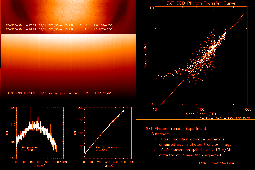
The figure given in the upper right is a photon transfer curve of the SXT CCD.
The crosses are from the bottom half of the CCD and the diamonds are from the
top half.  The two, nearly identical, straight lines have been fitted to the
middle portion (signal 100-275 DN, slope =1.2) of the bottom points and to all
of the top points.

This work yields the surprising (alarming?) result that the camera gain on
22-24 April 1998 was 13 electrons/DN -- 1/7 of the pre-launch gain setting.
This is a PRELIMINARY result and should not be taken too seriously until what
I've done has been validated by experts.  The last attempt to determine CCD
camera gain was by Barry LaBonte and is reported in

	show_pix/calibration/sxt_ccd_gain.

Barry concluded, using a different technique, that the camera gain in June
1996 was 87.9 +/- 1.4 electrons per DN.

The photon transfer curve technique is one of the most powerful means of
determining the performance of a CCD camera system.  In this technique the
signal variance (ordinate) is plotted versus the signal in DN (abcissa) on a
log-log plot.  I processed the data from the bottom and top FR images in two
different ways.  The problem in such an analysis is to minimize contributions
to the variance from fixed-pattern noise.  In the case of the bottom half of
the CCD I had two images so I got the signal from the sum of the 2 images and
the variances from their difference.  This permitted me to the sort the
signals by intensity (DN) and compute the variance from the difference image
for each of these sortings.  For the top-half case I only had a single photon
transfer image so I computed the average signal and the variance for 61
columns (460:520) around the flat top of the illumination of the CCD, for each
row of the image.  This greatly increased the scatter but the result is in
agreement with the analysis of the bottom half.  The IDL code used for this
purpose is appended to this message.

It is difficult to believe that the camera gain has shifted to such a high
value.  This would mean that our absolute solar intensities are off by the same
factor of 7, i.e., a factor of 7 too large.  Also, the pre-launch system gain
was adjusted so that the CCD would saturate (exceed full-well capacity) before
the ADC saturates for FR operation.  This level, about 235 DN does not
appear to have changed significantly.   I hope that someone can help me to
undestand what is going on here!

						L. Acton
						2 Oct 1998

++++++++++++++++++++++++++++++++++++++++++++++++++++++++++++++++++++++++
;10/02/98
;Photon Transfer Curve Analysis
;Data:
;  12 22-SEP-98  22:38:06  QT/M  NaBan/Open  Full Dark L   2     1.0 1024x512
;  13 22-SEP-98  23:10:06  QT/H  Open /AlMg  Full Dark L   2     1.0 1024x512
;  17 23-SEP-98  00:50:36  QT/H  NaBan/Open  Full Dark L   2     1.0 1024x512
;  20 24-SEP-98  00:36:40  QT/H  NaBan/Open  Full Dark L   2     1.0 1024x512
;  21 24-SEP-98  01:08:44  QT/H  Open /AlMg  Full Dark L   2     1.0 1024x512
;  22 24-SEP-98  01:13:00  QT/H  Open /AlMg  Full Dark L   2     1.0 1024x512

;READ THE DATA
rd_sda,'ccd_phot_xfer.sda',-1,index,data

;PROCESS THE 'BOTTOM HALF' IMAGES
noise=float(data(*,*,12))-data(*,*,20)
signal=(float(data(*,*,12))-data(*,*,13))+$
   (float(data(*,*,20))-data(*,*,21))

;EXCLUDE EDGES AND BLEMS
okx=indgen(1021)+2
okx=delind(okx,[366,601])
oky=indgen(502)+10

cleansig=fltarr(1019,502)
for i=0,501 do cleansig(*,i)=signal(okx,oky(i))
cleannoise=fltarr(1019,502)
for i=0,501 do cleannoise(*,i)=noise(okx,oky(i))

;ANALYZE THE 'BOTTOM' PHOTON TRANSFER DATA, SORTED BY SIGNAL LEVEL
;    SET UP THE PROCESSING PARAMETERS AND THE ARRAYS
h=histogram(cleansig)
n = n_elements(h)
pp=where(cleansig gt 0)
amin = min(cleansig(pp))
x = findgen(n) + long(amin)
xxx=fltarr(max(x)-min(x)+1)   ;SIGNAL ARRAY
yyy=fltarr(max(x)-min(x)+1)   ;VARIANCE ARRAY
nnn=lonarr(n_elements(x))     ;"NUMBER OF SAMPLES" ARRAY

for i=fix(amin),fix(max(x)) do begin
  j=i-fix(amin)
  ii=where(long(cleansig) eq i,nn)
  nnn(j)=nn
  if (nn ge 400) then begin
    xxx(j)=total(cleansig(ii))/nn
    yyy(j)=(stddev(cleannoise(ii)))^2
  endif
endfor

jj=where(xxx gt 0)
xxx=xxx(jj)
yyy=yyy(jj)

;PROCESS THE 'TOP HALF' IMAGES
topsig=float(data(okx,oky,17))-data(okx,oky,22)

xxxt=fltarr(n_elements(oky))  ;SIGNAL ARRAY
yyyt=fltarr(n_elements(oky))  ;VARIANCE ARRAY

for i=0,n_elements(oky)-1 do begin
   xxxt(i)=mean(topsig(460:520,i))   ;CHOOSE 60 COLUMNS FROM FLAT TOP OF
   yyyt(i)=(stddev(topsig(460:520,i)))^2   ;OF THE INTENSITY DISTRIBUTION
endfor

;PLOT THE RESULTS
wdef,1,450
plot_oo,xxx,yyy,$
   xtit='Mean Signal (DN)',$
   ytit='Variance (DN)',psym=1,symsiz=0.5,$
   tit='SXT CCD Photon Transfer Curve',$
   charsize=1.3
oplot,xxxt,yyyt,psym=4,symsiz=0.4

plottime

;FIT AND PLOT A CURVE TO THE CENTRAL PORTION OF THE 'BOTTOM' CURVE
ii=where(xxx ge 100 and xxx le 275)
sln=poly_fit(alog10(xxx(ii)),alog10(yyy(ii)),1,sfit)
;print,sln
;    -0.701368
;     0.500844

aa=1000
bb=10^(sln(0)+(sln(1)*alog10(aa)))
aa=1
cc=10^(sln(0)+(sln(1)*alog10(aa)))
oplot,[1,1e3],[cc,bb],color=100

;FIT AND PLOT A CURVE TO THE 'TOP' RESULTS (DIAMONDS)
sln=poly_fit(alog10(xxxt),alog10(yyyt),1,tyfit)
;print,sln
;    -0.581393
;     0.514919
aa=1000
bb=10^(sln(0)+(sln(1)*alog10(aa)))
aa=1
cc=10^(sln(0)+(sln(1)*alog10(aa)))
oplot,[1,1e3],[cc,bb]

end