Attention EIT software users
The calling syntax of eit_prep has just changed and the new version is NOT backwards compatible. Please modify your programs according to the update instructions.
This is the most basic operation. To check if the fits file is not a multiple fits file, try
IDL> print, eit_fxpar(hdr, 'NAXIS3')
If NAXIS3 greater than 1, go to Dealing with Multi-image fits file. Anyhow, if you've got a single-image fits file, and if you want to obtain the image data, you could do:
IDL> img = readfits(file, hdr)
which will read the data directly from the fits file and return the EIT header information. However, this method is not recommended. It is better to always make use of the eit_prep.pro program.
|
Attention EIT software users The calling syntax of eit_prep has just changed and the new version is NOT backwards compatible. Please modify your programs according to the update instructions. |
If you'd like to have the data properly calibrated (i.e. flat-fielded, degridded, exposure time normalized to DN [data numbers] per second, filter normalized, and response normalized), there is a program called eit_prep.pro. This program should be used whenever possible since its source code is regularly updated to include the latest developpements of the calibration. (For descriptions of exposure time and filters, see header information). To read in a single-image EIT FITS file, use eit_prep like so:
IDL> eit_prep, file, header, image
which reads the specified FITS file, analyzes the content of the header and applies all the relevant calibrations. These include
Dark current subtraction: a uniform (identical for all the pixels) zero flux response is subtracted from the raw image. Since this is a time-varying function, always make sure you have the latest version of eit_dark.pro.
Degridding : the aluminum filter located close to the focal plane of the instrument casts a shadow on the CCD detector that creates a modulation pattern, or "grid", in the images. The degridding factors were calculated and stored in the software tree, and the image is multiplied by the degridding factor for a fairly reasonable correction to the data.
Filter normalization: account is taken for the variable transmittivity of the clear and aluminum filters (Al+1 or Al+2).
Exposure time normalization: the flux is normalized to the exposure time. Binned images are treated properly.
Response correction: due to exposure to EUV flux, the pixel to pixel sensitivity (flat-field) of the CCD detector is higly variable. The flat-fields needed to correct the images are computed regularly from images of visible light calibration lamps. Since this correction is a time-dependent variable, the response factor may not (yet) have been calculated for the most recent dates. Please go to this page to make sure that you have the most recent calibration lamps in your local database and that your software is up to date.
A few other corrections (vignetting, stray-light) will be added soon. For more details, see the calibration section of this guide.
If you wish you can various keywords to your call to eit_prep in order to control the level of calibration applied to the data:
IDL> eit_prep, file, header, image, /no_calibrate
this will return a raw image with no calibration applied at all. It is equivalent to the simple use of read_fits described above.
If the file you are dealing with is a multiple-image file, you can process a single image, a vector, or all the images:
Single image: IDL> eit_prep, file, hdrs, datacube, image_no=3, /save_zero Vector: IDL> eit_prep, file, hdrs, datacube, image_no=[0,5,22], /save_zero All the images: IDL> eit_prep, file, hdrs, datacube, image_no='all', /save_zero
If all of the data is missing in a single image, the keyword /save_zero forces eit_prep to return a blank image (normally it would just return a zero, which won't fit into your data cube). You now have a processed data cube - the images may be of different wavelengths, you can check:
IDL> print, eit_fxpar(hdr, 'WAVELNTH', image_no=5)
which returns the wavelength of the fifth image in the data cube. You can also return an array of all of the wavelengths:
IDL> waves = eit_fxpar(hdr, 'WAVELNTH', image_no='all')
IDL> read_eit, filelist, inhdr, imgs
IDL> eit_prep, inhdr, outhdr, imgs, data=temporary(imgs)
Often one might wish to process a number of FITS files without saving all the data in memory but rather writing the processed data to new FITS files. This is accomplished via:
IDL> mk_eit_l1, list = filelist
You may wish to examine the other options for this routine.
IDL> tvscl, alog10(img>0.5)
where img is two-dimensional. If you've got several images in a data cube, you can do
IDL> tvscl, alog10(img[*,*,5]>0.5)
which will display the 6th image of the cube. Since there may be pixels with zero counts in the image, the image is floored with a value of 0.5 before taking its logarithm. Setting a lower bound avoids errors generated when trying to compute the non-defined value of the logarithm of zero. Experiment by varying the lower and upper limits until the image looks best. Note: images with the same wavelength should be displayed with the same upper and lower limits if they are to be compared.
IDL> wave = eit_fxpar(hdr, 'WAVELNTH')
or
IDL> wave = eit_fxpar(hdr, 'WAVELNTH', image_no=5)
IDL> eit_colors, wave
You could also do:
IDL> xloadct, file = getenv('coloreit')
to get the color table widget.
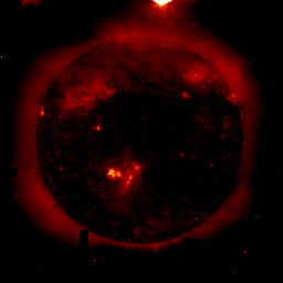
For example, the image on the left is an EIT 284 Å displayed with the Red Temperature table (bad!) without playing with the lower and upper limits:
IDL> tvscl, alog10(img>0.5)
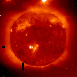
While the image in the middle is displayed with better limits but in the wrong color table:
IDL> tvscl, alog10(img>0.02<50)
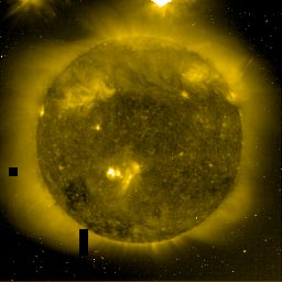
while the final image (which shows much better quiet sun detail because the color table is optimized for an EIT image in that particular wavelength) is both scaled properly and has the correct color table:
 |
 |
 |
This section is not meant to be an exhaustive study of EIT pointing questions, but rather to introduce the User to the main parameters and PITFALLS, especially with regards to co-alignment with other instruments. It is assumed the user is familiar with the standard FITS keywords, CRPIX, CRVAL, etc. NOTE, FITS standard starts with pixel (1,1) while IDL uses pixel (0,0). you may need to correct for this.
WHERE ARE WE POINTED? Not an easy question. Until recently, EIT had used automated limb-fitter to determine the Solar pointing. As is well known, this method can fail given the presence of above-limb material. The level zero data has been re-processed with a more accurate determination of the pointing. For older data, you can obtain the pointing of EIT, by ignoring the FITS headers and using the function eit_point, e.g.
IDL> xy = eit_point(date, wavelength)
An additional complication is subfield images taken prior to the re-processing date. These images contain no values of CRPIX, CRVAL, but instead have the "raw" pixel coordinates, (P1_X:P2_X,P1_Y:P2_Y). To convert these to Solar coordinates one must get the xy pointing as above and then to obtain the lower left corner of the image:
IDL> CRPIX1 = (eit_fxpar(hdr,'p1_x')-xy(0)-1) * eit_pixsize()
IDL> CRPIX2 = (eit_fxpar(hdr,'p1_y')-xy(1)-20) * eit_pixsize()
EXPOSURE TIME: The time given in the header reflects the commanded exposure time plus a SHUTTER DWELL TIME which is approximately 2.1 seconds. Due to on-board software problems, this shutter time is not properly reflected in the images prior to July 17, 1996 and has been fixed at 2.1 seconds.
OBSERVATION TIME: Here again, there is an ambiguity due to the on-board software. The time reflected in the DATE_OBS field is the "nominal" start time of the exposure. HOWEVER, we realized that this time was off from the "true" start time, by varying amounts up to 5 minutes. Starting from September 1997, a better approximation to the "true" start time is given in the CORRECTED DATE_OBS field (mapped to CORR_OBS in structures)l this time should be within ~ 15 s of the actual UTC of the start of the exposure. This may be important when performing detailed time comparisons, e.g. high cadence EIT images versus MDI hi-res magnetograms.
Last revised: 2006 June 17 - J.B. Gurman