The calibration of EIT is very complex, and getting it right was a lenghty process. The calibration is now in its final phase, meaning that only minor software modifications or additions will occur. On the way towards the present calibration, numerous versions of the software were produced, each reflecting the knowledge of the time. Here is a brief history of the successive updates.
| 1999 May 12 | Calibration and software updated |
| 1999 June 09 | Bug fix for Emission measure calculation via EIT_TEMP.PRO |
| 1999 Nov. 17 | Calibration and software updated |
| 2000 Jan. 05 | Relative response normalization and call to EIT_PREP.PRO updated |
| 2001 June 11 | Online calibration and associated software (EIT_PREP is top level) updated. New calibration lamp database online |
| 2001 Dec. 10 | New calibration and software are online |
Note that since the calibration is time-dependant, a few routines in the EIT software are regularly updated in order to reflect he changes occuring in the instrument. Therefore, you need to check periodically if you have the lastest version of some routines.
This chapter is meant to be used as a brief guide to EIT calibration. The calibration will be discussed in terms of relative (time variability) and absolute calibration. The use of SOHO EIT observations as a diagnostic for temperature, density or irradiance measurements depends upon a reliable photometric calibration. We discuss here the present state of this calibration.
An initial calibration was given by Delaboudinière et al. (1995) and incorporated into the analysis software as part of the SolarSoftWare package. This is the calibration used in all previous EIT papers. This calibration relied on part by some modelling and as well as measurements of the witness mirrors instead of the flight mirrors. The main calibration data were obtained with the Orsay synchrotron and presented in the Ph.D. thesis of Song (1995). This data set is believed to contain a more realistic calibration. The Song data has been re-analyzed in two separate works, first that of Defise (1999, Ph.D.) and by Dere et al. (2000). The calibration work by Dere is a more detailed examination of the pre-flight calibration. This work is presented in Dere et al. 2000. Comparisons of Dere's with other calibrations are not yet available.
The online software has been updated on November 17, 1999 to reflect a modified version of the Dere calibration. The modifications include the far wings of the bandpass and a probably more correct treatment of the second order He II for the 304 bandpass. Note, for almost all work, these modifications have a negligible effect on the final output. To graphically view the calibration see Calib.ps. The solid lines in this plot are the Dere calibration, while the dashed are the modifications. This modified calibration is presented in Cook et al., 2002.
In addition to these pre-flight calibration updates, work has been done using the in-flight data. In particular, an in-flight measurement of the photons/DN conversion was made by Moses et al. (1999) which will replace the theoretical conversion used in old calibrations. This will be incorporated with the post-flight calibration updates. A final photometric comparison with the Naval Research Lab EIT CalRoc (Moses et al., 2000) is still pending. It should be noted that these are changes in the photometric calibrations and do not change any conclusions based upon relative changes.
| Sector | Plots | |
|---|---|---|
| Fe IX/X 171 Å | Linear | |
| Fe XII 195 Å | Linear | |
| Fe XV 284 Å | Linear | |
| He II 304 Å | Linear | |
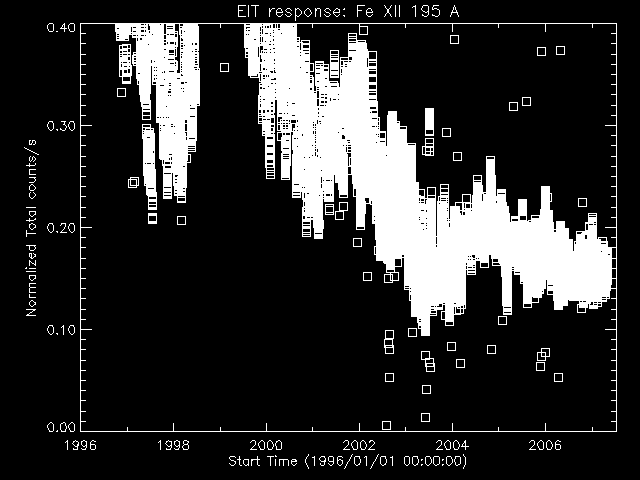
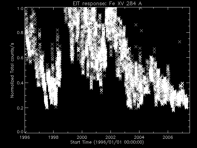
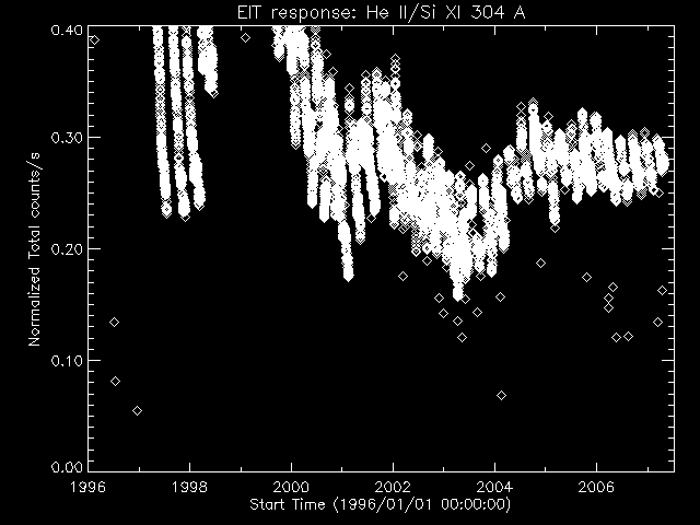
As is well known, the response of the EIT CCD has changed with time. The variation of the instrument throughput is monitored by the total flux in a full field image for each bandpass. A detailed discussion of this and the following brief comments can be found in Moses et al. 1997. The utility of this monitor is determined by the variability of the solar flux in each waveband. The intrinsic solar variability increases with the temperature of the dominant emission line the bandpass. Thus the monitor is very good for the 304 (He II) and the 171 (Fe X,IX) channels where the solar variability is low, while it degrades for the 195 (Fe XII) channel and is useless for the 284 (Fe XV) channel where changes in the instrumental response are masked by solar changes. Since the extremes of the wavelength regime are 171 and 304, this technique allows the full wavelength dependence of the degradation to be monitored.
Since the 304 channel is the most sensitive to degradation, it best illustrates the processes. The initial increase in response over the first month of observations is attributed to an overall outgassing of the instrument. In order to reverse the subsequent decline in response, the CCD was heated (baked out) to 18C on 23 May 1996. Initial recovery was to the highest throughput observed in flight. Successive heat cycles were conducted according to the requirements of the observing schedules and in exploration of the causes of the decline. The degradation process consists of several components which are difficult to separate in detail. The two basic processes contributing to the degradation are 1) the absorption of EUV before it interacts with the CCD by a surface contaminant and 2) the reduction of charge collection efficiency (CCE) in the CCD due to EUV induced device damage.
Many users of EIT data wish to know the conversion from DNs from physical units of flux or intensity, i.e. photons.m-2.sec-1.sr-1 or Watts.m-2.sr-1. This is not a trivial as one would hope. The main complication, is that EIT is not a spectrometer but a broad band (FWHM ~10 Å) instrument containing various emission lines formed at various temperatures in each bandpass. As the response for each bandpass is not a square well, each line contributes a different amount of the total flux, according to the relative response and strength of the lines. Therefore, there is no unique transformation of DNs to units of flux! Instead, it depends upon the Differential Emission Measure (DEM) of the formation region and knowledge of the instrument response.
How do we proceed? There are a couple of ways to move forward. In terms of the instrumental response, one can make assumptions (e.g. square well, dominance of some lines) or one can use the actual response. As for the line formation, we can proceed in two ways. The DEM of a region of interest may be known from another source, e.g. averages given as part of the CHIANTI package or CDS, SERTS, etc, measurements. Then one can use a spectral package (CHIANTI) combined with the DEM bandpass information to produce a synthetic spectrum. This gives you the absolute flux in terms of real units. A different method presently being developed (Cook et al. 2002) is to use the EIT data itself to compute a rough DEM curve and then the conversion to real units.
The one exception to this is the 304 bandpass. This bandpass is dominated by He II (70-95% on disk depending on type of region) while most of the remainder of the flux is due to the nearby Si XI line (dominant off disk), which therefore has the same instrumental response. Therefore, conversion of DNs to intensity for this bandpass is fairly straightforward.
Last revised: Tuesday, December 25, 2001 2:01 PM - F. Auchère